The impedance behavior of a purely capacitive coating was discussed above. Most paint coatings degrade with time, resulting in more complex behavior.
After a certain amount of time, water penetrates into the coating and forms a new liquid/metal interface under the coating. Corrosion phenomena can occur at this new interface.
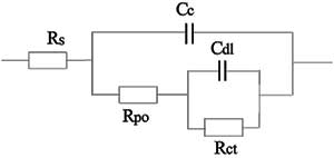
The impedance of coated metals has been extensively studied. The interpretation of impedance data from failed coatings can be very complicated so only the simple equivalent circuit shown in Figure 22 will be discussed here. Even this simple model has been the cause of some controversy in the literature. Researchers do not agree on the assignment of impedances to physical processes that can occur in the cell. The discussion below is therefore only one of several interpretations of this model.
Gamry scientists published three articles on the evaluation of organic coatings with EIS in JCT CoatingsTech (www.coatingstech.org). The articles are:
Fundamentals of Electrochemical Impedance Spectroscopy, August 2004.
Application of EIS to Coatings, October 2004.
Protocols for Testing Coatings with EIS, February 2005.
The capacitance of the intact coating is represented by Cc. Its value is much smaller than a typical double layer capacitance. Its units are pF or nF, not μF. Rpo (pore resistance) is the resistance of ion conducting paths the develop in the coating. These paths may be physical pores filled with electrolyte. On the metal side of the pore, we assume that an area of the coating has delaminated and a pocket filled with an electrolyte solution has formed. This electrolyte solution can be very different than the bulk solution outside of the coating. The interface between this pocket of solution and the bare metal is modeled as a double-layer capacitance in parallel with a kinetically controlled charge-transfer reaction.

Figure 22. Equivalent Circuit for a Failed Coating
When you use EIS to test a coating, you fit a data curve to this type of model. The fit returns estimates for the model parameters, such as the pore resistance and the double layer capacitance. You then use these parameters to evaluate the degree to which the coating has failed.
In order to show realistic data curves, we need to do this operation in reverse. Assume that we have a 10 cm2 sample of metal coated with a 12 μm film. Assume that we have five delaminated areas making up a total of 1% of the surface of the metal. The pores in the film that give access into these delaminated areas can be represented as being solution filled cylinders, with a 30 μm diameter.
The parameters used to develop the curves are shown below:
Cc= 4 nF | (Calculated for 10 cm2 area, εr = 6 and 12 μm thickness) |
Rpo = 3400 Ω | (Calculated assuming κ (conductivity) = 0.01 S/cm) |
Rs= 20 Ω | (Assumed) |
Cdl= 4 μF | (Calculated for 1% of 10 cm2area and assuming 40 μF/cm2) |
Rct = 2500 Ω | (Calculated for 1% of 10 cm2area and using Polarization Resistance assumptions from an earlier discussion) |
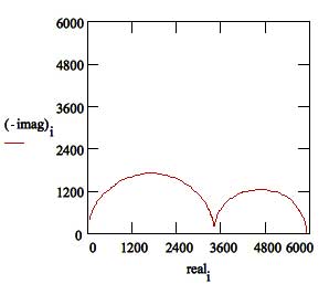
With these parameters, the Nyquist Plot for this model is shown in Figure 23. Notice that there are two time constants in this plot.

Figure 23. Nyquist Plot for a Failed Coating
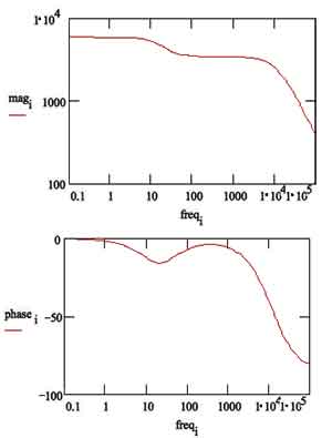
The Bode Plot of the same data is shown in Figure 24. The two time constants are not nearly as pronounced on this plot. The plot does not go sufficiently high in frequency to measure the solution resistance. In practice this is not a problem, because the solution resistance is a property of the test solution and the test cell geometry, not a property of the coating. It is, therefore, not very interesting.

Figure 24. Bode Plot for a Failed Coating
Extracting Model Parameters from Data
Modeling Overview
EIS data are generally analyzed in terms of a equivalent circuit model. Echem Analyst tries to find a model whose impedance matches the measured data.
The type of electrical components in the model and their interconnections control the shape of the model's impedance spectrum. The model's parameters (e.g., the resistance value of a resistor) control the size of each feature in the spectrum. Both these factors affect the degree to which the model's impedance spectrum matches a measured EIS spectrum.
In a physical model, each of the model's components is postulated to come from a physical process in the electrochemical cell. All of the models discussed earlier in this chapter are physical models. The choice of which physical model applies to a given cell is made from knowledge of the cell's physical characteristics. Experienced EIS analysts can also use the shape of a cell's EIS spectrum to help choose a model for that cell.
Models can also be partially or completely empirical. The circuit components in this type of model are not assigned to physical processes in the cell. The model is chosen to give the best possible match between the model's impedance and the measured impedance.
An empirical model can be constructed by successively subtracting component impedances from a spectrum. If the subtraction of an impedance simplifies the spectrum, the component is added to the model, and the next component impedance is subtracted from the simplified spectrum. This process ends when the spectrum is completely gone.
As we shall see below, physical models are generally preferable to empirical models.
Non-linear Least Squares Fitting
Modern EIS analysis uses a computer to find the model parameters that cause the best agreement between a model's impedance spectrum and a measured spectrum. A non-linear least squares fitting (NLLS) algorithm is used.
NLLS starts with initial estimates for all the model's parameters. Starting from this initial point, the algorithm makes a change in one of the parameter values and evaluates the resulting fit. If the change improves the fit, the new parameter value is accepted. If the change worsens the fit, the old parameter value is retained. Next, a different parameter value is changed and the test is repeated. Each trial with new values is called an iteration. Iterations continue until the goodness of fit exceeds an acceptance criterion, or until the number of iterations reaches a limit.
NLLS algorithms are not perfect. In some cases they do not converge on a useful fit. This can be the result of several factors including:
An incorrect model for the data set being fitted.
Poor estimates for the initial values.
Noise
In addition, the fit from an NLLS algorithm can look poor when the fit's spectrum is superimposed on the data spectrum. It appears as though the fit ignores a region in the data. To a certain extent this is what happens. The NLLS algorithm optimizes the fit over the entire spectrum. It does not care that the fit looks poor over a small section of the spectrum.